25 Handling Missing data

Missing data is a very common issue in statistics and data science.

Data may be missing for a variety of reasons. We often characterize the type of missingness using the following three types (Mack, Su, and Westreich 2018):

Missing completely at random (MCAR): “The fact that the data are missing is independent of the observed and unobserved data”
Missing at random (MAR): “The fact that the data are missing is systematically related to the observed but not the unobserved data”
Missing not at random (MNAR): “The fact that the data are missing is systematically related to the unobserved data”

25.1 Check for missing data

You can use your favorite base R commands to check for missing data, count NA elements by row, by column, total, etc.

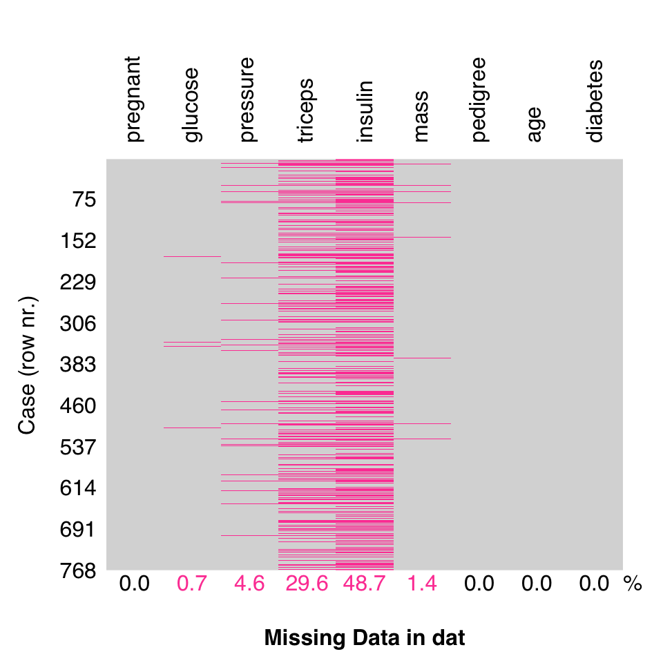
Let’s load the PimaIndiansDiabetes2 dataset from the mlbench package and make a copy of it to variable dat. Remember to check the class of a new object you didn’t create yourself with class(), check its dimensions, if applicable, with dim(), and a get a summary of its structure including data types with str():

data("PimaIndiansDiabetes2", package = "mlbench")
dat <- PimaIndiansDiabetes2
class(dat)

[1] "data.frame"

dim(dat)

[1] 768   9

str(dat)

'data.frame':   768 obs. of  9 variables:
 $ pregnant: num  6 1 8 1 0 5 3 10 2 8 ...
 $ glucose : num  148 85 183 89 137 116 78 115 197 125 ...
 $ pressure: num  72 66 64 66 40 74 50 NA 70 96 ...
 $ triceps : num  35 29 NA 23 35 NA 32 NA 45 NA ...
 $ insulin : num  NA NA NA 94 168 NA 88 NA 543 NA ...
 $ mass    : num  33.6 26.6 23.3 28.1 43.1 25.6 31 35.3 30.5 NA ...
 $ pedigree: num  0.627 0.351 0.672 0.167 2.288 ...
 $ age     : num  50 31 32 21 33 30 26 29 53 54 ...
 $ diabetes: Factor w/ 2 levels "neg","pos": 2 1 2 1 2 1 2 1 2 2 ...

Check if there are any missing values in the data.frame with anyNA():

anyNA(dat)

[1] TRUE

The above suggests there is one or more NA values in the dataset.

We can create a logical index of NA values using is.na(). Remember that the output of is.na() is a logical matrix with the same dimensions as the dataset:

na_index <- is.na(dat)
dim(na_index)

[1] 768   9

head(na_index)

  pregnant glucose pressure triceps insulin  mass pedigree   age diabetes
1    FALSE   FALSE    FALSE   FALSE    TRUE FALSE    FALSE FALSE    FALSE
2    FALSE   FALSE    FALSE   FALSE    TRUE FALSE    FALSE FALSE    FALSE
3    FALSE   FALSE    FALSE    TRUE    TRUE FALSE    FALSE FALSE    FALSE
4    FALSE   FALSE    FALSE   FALSE   FALSE FALSE    FALSE FALSE    FALSE
5    FALSE   FALSE    FALSE   FALSE   FALSE FALSE    FALSE FALSE    FALSE
6    FALSE   FALSE    FALSE    TRUE    TRUE FALSE    FALSE FALSE    FALSE

One way to count missing values is with sum(is.na()). Remember that a logical array is coerced to an integer array for mathematical operations, where TRUE becomes 1 and FALSE becomes 0. Therefore, calling sum() on a logical index counts the number of TRUE elements (and since we are applying it on the index of NA values, it counts the number of elements with missing values):

sum(is.na(dat))

[1] 652

There are 652 NA values in total in the data.frame.

Let’s count the number of missing values per feature, i.e. per column, using sapply():

sapply(dat, function(i) sum(is.na(i)))

pregnant  glucose pressure  triceps  insulin     mass pedigree      age 
       0        5       35      227      374       11        0        0 
diabetes 
       0

The features insulin and triceps have the most NA values.

Let’s count the number of missing values per case, i.e. per row:

sapply(1:nrow(dat), function(i) sum(is.na(dat[i, ])))

  [1] 1 1 2 0 0 2 0 3 0 3 2 2 2 0 0 3 0 2 0 0 0 2 2 1 0 0 2 0 0 2 1 0 0 2 1 0 2
 [38] 1 1 0 0 2 1 0 2 1 2 1 1 4 0 0 0 0 0 1 0 0 2 0 4 2 2 0 2 1 1 2 0 0 0 0 2 0
 [75] 1 2 2 1 3 1 1 4 0 1 2 0 1 0 0 1 2 0 0 2 0 0 1 0 0 0 2 2 2 0 2 0 2 0 0 0 0
[112] 0 0 2 0 2 2 2 1 0 0 1 0 2 2 0 0 0 0 2 0 2 0 1 0 0 0 0 2 0 2 1 0 2 0 2 1 0
[149] 2 1 0 2 0 0 2 1 0 0 0 0 1 0 0 1 2 0 1 2 2 0 2 0 2 0 0 0 2 0 2 2 2 0 1 2 2
[186] 1 0 0 0 0 2 0 2 3 1 0 2 0 0 0 1 2 1 0 0 1 0 2 0 1 1 1 1 0 0 0 0 0 1 2 0 2
[223] 3 0 0 0 2 1 0 0 2 0 0 2 0 2 0 1 1 2 1 0 2 0 0 1 2 0 0 1 2 2 0 1 0 1 1 1 0
[260] 0 0 3 1 1 2 0 3 1 2 3 1 0 2 0 2 0 1 0 2 0 2 0 0 2 2 0 0 0 0 0 0 0 0 0 2 0
[297] 0 0 0 2 3 0 0 2 2 0 0 0 0 0 1 0 0 0 1 0 0 2 0 2 0 1 1 0 1 0 0 2 0 0 1 0 3
[334] 2 0 0 3 2 0 2 0 0 2 2 2 0 0 3 0 2 2 2 1 0 2 2 0 2 0 0 0 2 1 2 0 0 2 1 0 0
[371] 0 1 0 0 0 0 0 0 2 0 0 1 0 0 0 0 1 1 0 0 0 2 0 0 2 0 0 1 2 1 2 2 0 1 2 0 2
[408] 2 2 0 1 0 0 0 0 0 1 1 2 0 0 0 0 1 0 0 4 0 0 0 3 0 0 2 1 3 1 2 1 2 1 0 0 2
[445] 1 0 0 0 0 0 0 2 0 3 0 1 2 0 0 0 0 2 0 1 2 0 0 0 3 0 1 1 1 2 2 1 0 0 0 1 0
[482] 1 0 0 3 0 0 0 1 2 0 1 1 0 4 2 2 0 0 0 0 1 2 0 1 2 0 0 0 2 1 0 2 2 0 0 0 2
[519] 2 0 0 0 4 2 2 1 0 0 0 2 0 2 0 3 0 3 2 2 0 0 0 0 1 0 0 0 0 0 0 1 1 0 2 0 0
[556] 0 1 2 1 2 2 0 0 0 2 0 0 0 0 0 2 2 0 0 0 0 0 2 2 1 1 1 1 2 0 1 2 2 0 3 1 0
[593] 2 0 0 0 2 0 2 0 1 3 1 0 3 1 0 0 0 0 0 0 0 1 0 2 2 0 1 3 0 1 2 0 2 0 2 2 2
[630] 1 2 0 2 0 2 2 2 0 0 0 0 2 2 3 0 0 0 0 0 1 0 0 0 2 0 0 0 0 2 0 2 1 0 0 1 0
[667] 1 1 0 0 0 1 0 0 2 2 2 2 2 0 0 1 0 2 3 0 2 1 0 0 2 2 0 0 2 0 0 3 0 2 0 1 1
[704] 3 0 1 4 0 2 0 0 0 1 0 2 0 0 1 0 1 1 0 0 0 2 1 0 1 2 2 0 2 0 0 2 1 0 1 0 2
[741] 0 0 0 2 0 0 1 0 0 2 2 0 1 0 1 0 1 2 2 2 0 1 2 0 1 0 2 1

If we wanted to get the row with the most missing values, we can use which.max():

which.max(sapply(1:nrow(dat), function(i) sum(is.na(dat[i, ]))))

[1] 50

sum(is.na(dat[50, ]))

[1] 4

Row 50 has 4 missing values.

25.1.1 Visualize

It may be helpful to visualize missing data to get a quick impression of missingness. The rtemis package includes the function mplot3_missing():

library(rtemis)

  .:rtemis 0.95.6 🌊 aarch64-apple-darwin20 (64-bit)

mplot3_missing(dat)

Missing data is shown in magenta by default. The row below the image shows total NA values per column

25.1.2 Summarize

Get number of missing values per column:

sapply(dat, function(i) sum(is.na(i)))

pregnant  glucose pressure  triceps  insulin     mass pedigree      age 
       0        5       35      227      374       11        0        0 
diabetes 
       0

rtemis::check_data() includes information on missing data:

check_data(dat)

  dat: A data.table with 768 rows and 9 columns

  Data types
  * 8 numeric features
  * 0 integer features
  * 1 factor, which is not ordered
  * 0 character features
  * 0 date features

  Issues
  * 0 constant features
  * 0 duplicate cases
  * 5 features include 'NA' values; 652 'NA' values total
    * 5 numeric

  Recommendations
  * Consider imputing missing values or use complete cases only

25.2 Handle missing data

Different approaches can be used to handle missing data:

Do nothing - if your algorithm(s) can handle missing data (decision trees!)
Exclude data: Use complete cases only
Fill in (make up) data: Replace or Impute
- Replace with median/mean
- Predict missing from present
  - Single imputation
  - Multiple imputation

25.2.1 Do nothing

Algorithms like decision trees and ensemble methods that use decision trees like random forest and gradient boosting can handle missing data, depending on the particular implementation. For example, rpart::rpart() which is used by rtemis::s_CART() has no trouble with missing data in the predictors:

dat.cart <- s_CART(dat)

09-28-23 21:48:19 Hello, egenn [s_CART]

09-28-23 21:48:19 Imbalanced classes: using Inverse Frequency Weighting [dataPrepare]

.:Classification Input Summary
Training features: 768 x 8 
 Training outcome: 768 x 1 
 Testing features: Not available
  Testing outcome: Not available

09-28-23 21:48:20 Training CART... [s_CART]

.:CART Classification Training Summary
                   Reference 
        Estimated  neg  pos  
              neg  426   89
              pos   74  179

                   Overall  
      Sensitivity  0.8520 
      Specificity  0.6679 
Balanced Accuracy  0.7600 
              PPV  0.8272 
              NPV  0.7075 
               F1  0.8394 
         Accuracy  0.7878 
              AUC  0.7854 

  Positive Class:  neg 
09-28-23 21:48:20 Completed in 0.01 minutes (Real: 0.43; User: 0.41; System: 0.02) [s_CART]

25.2.2 Use complete cases only

R’s builtin complete.cases() function returns, as the name suggests, a logical index of cases (i.e. rows) that have no missing values, i.e. are complete.

dim(dat)

[1] 768   9

index_cc <- complete.cases(dat)
class(index_cc)

[1] "logical"

length(index_cc)

[1] 768

head(index_cc)

[1] FALSE FALSE FALSE  TRUE  TRUE FALSE

dat_cc <- dat[index_cc, ]
dim(dat_cc)

[1] 392   9

We lost 376 cases in the above example. That’s quite a few, so, for this dataset, we probably want to look at options that do not exclude cases.

25.2.3 Replace with a fixed value

We can manually replace missing values with the mean or median in the case of a continuous variable, or with the mode in the case of a categorical feature.
For example, to replace the first feature’s missing values with the mean:

pressure_mean <- mean(dat$pressure, na.rm = TRUE)
dat_im <- dat
dat_im$pressure[is.na(dat_im$pressure)] <- pressure_mean

rtemis::preprocess() can replace missing values with mean (for numeric features) and the mode (for factors) for all columns:

dat_pre <- preprocess(dat, impute = TRUE, impute.type = "meanMode")

09-28-23 21:48:20 Preprocessing dat... [preprocess]
09-28-23 21:48:20 Imputing missing values using mean and get_mode... [preprocess]
09-28-23 21:48:20 Completed in 0.00 minutes (Real: 0.00; User: 1e-03; System: 0.00) [preprocess]

Verify there are no missing data by rerunning check_data():

check_data(dat_pre)

  dat_pre: A data.table with 768 rows and 9 columns

  Data types
  * 8 numeric features
  * 0 integer features
  * 1 factor, which is not ordered
  * 0 character features
  * 0 date features

  Issues
  * 0 constant features
  * 0 duplicate cases
  * 0 missing values

  Recommendations
  * Everything looks good

You may want to include a “missingness” column that indicates which cases were imputed to include in your model. You can create this simply by running:

pressure_missing = factor(as.integer(is.na(dat$pressure)))

preprocess() includes the option missingness to add indicator columns after imputation:

dat_pre <- preprocess(
    dat, 
    impute = TRUE, 
    impute.type = "meanMode",
    missingness = TRUE
)

09-28-23 21:48:20 Preprocessing dat... [preprocess]
09-28-23 21:48:20 Created missingness indicator for glucose... [preprocess]
09-28-23 21:48:20 Created missingness indicator for pressure... [preprocess]
09-28-23 21:48:20 Created missingness indicator for triceps... [preprocess]
09-28-23 21:48:20 Created missingness indicator for insulin... [preprocess]
09-28-23 21:48:20 Created missingness indicator for mass... [preprocess]
09-28-23 21:48:20 Imputing missing values using mean and get_mode... [preprocess]
09-28-23 21:48:20 Completed in 5e-05 minutes (Real: 3e-03; User: 3e-03; System: 0.00) [preprocess]

head(dat_pre)

  pregnant glucose pressure  triceps  insulin mass pedigree age diabetes
1        6     148       72 35.00000 155.5482 33.6    0.627  50      pos
2        1      85       66 29.00000 155.5482 26.6    0.351  31      neg
3        8     183       64 29.15342 155.5482 23.3    0.672  32      pos
4        1      89       66 23.00000  94.0000 28.1    0.167  21      neg
5        0     137       40 35.00000 168.0000 43.1    2.288  33      pos
6        5     116       74 29.15342 155.5482 25.6    0.201  30      neg
  glucose_missing pressure_missing triceps_missing insulin_missing mass_missing
1               0                0               0               1            0
2               0                0               0               1            0
3               0                0               1               1            0
4               0                0               0               0            0
5               0                0               0               0            0
6               0                0               1               1            0

25.2.3.1 Add new level “missing”

One option to handle missing data in categorical variables, is to introduce a new level of “missing” to the factor, instead of replacing with the mode, for example. If we bin a continuous variable to convert to categorical, the same can then also be applied.

Since no factors have missing values in the current dataset we create a copy and replace some data with NA:

dat2 <- dat
dat2$diabetes[sample(1:NROW(dat2), size = 35)] <- NA
sum(is.na(dat2$diabetes))

[1] 35

levels(dat2$diabetes)

[1] "neg" "pos"

Replace NA values with new level missing:

dat_pre2 <- preprocess(dat2, factorNA2missing = TRUE)

09-28-23 21:48:20 Preprocessing dat2... [preprocess]
09-28-23 21:48:20 Converting 1 factor's NA values to level 'missing'... [preprocess]
09-28-23 21:48:20 Completed in 0.00 minutes (Real: 0.00; User: 0.00; System: 0.00) [preprocess]

anyNA(dat_pre2$diabetes)

[1] FALSE

levels(dat_pre2$diabetes)

[1] "neg"     "pos"     "missing"

25.2.4 Last observation carried forward (LOCF)

In longitudinal / timeseries data, we may want to replace missing values with the last observed value. This is called last observation carried forward (LOCF). As always, whether this procedure is appropriate depend the reasons for missingness. The zoo and DescTools packages provide commands to perform LOCF.

Some simulated data. We are missing blood pressure measurements on Saturdays and Sundays:

dat <- data.frame(
     Day = rep(c("Mon", "Tues", "Wed", "Thu", "Fri", "Sat", "Sun"), times = 3),
     SBP = sample(105:125, size = 7 * 3, replace = TRUE)
)
dat$SBP[dat$Day == "Sat" | dat$Day == "Sun"] <- NA
dat

    Day SBP
1   Mon 123
2  Tues 124
3   Wed 116
4   Thu 125
5   Fri 118
6   Sat  NA
7   Sun  NA
8   Mon 121
9  Tues 117
10  Wed 109
11  Thu 121
12  Fri 121
13  Sat  NA
14  Sun  NA
15  Mon 116
16 Tues 111
17  Wed 110
18  Thu 118
19  Fri 110
20  Sat  NA
21  Sun  NA

The zoo package includes the na.locf().

dat$SBPlocf <- zoo::na.locf(dat$SBP)
dat

    Day SBP SBPlocf
1   Mon 123     123
2  Tues 124     124
3   Wed 116     116
4   Thu 125     125
5   Fri 118     118
6   Sat  NA     118
7   Sun  NA     118
8   Mon 121     121
9  Tues 117     117
10  Wed 109     109
11  Thu 121     121
12  Fri 121     121
13  Sat  NA     121
14  Sun  NA     121
15  Mon 116     116
16 Tues 111     111
17  Wed 110     110
18  Thu 118     118
19  Fri 110     110
20  Sat  NA     110
21  Sun  NA     110

Similar functionality is included in DescTools’ LOCF() function:

DescTools::LOCF(dat$SBP)

 [1] 123 124 116 125 118 118 118 121 117 109 121 121 121 121 116 111 110 118 110
[20] 110 110

25.2.5 Replace missing values with estimated values

25.2.5.1 Single imputation

You can use non-missing data to predict missing data in an iterative procedure (Buuren and Groothuis-Oudshoorn 2010; Stekhoven and Bühlmann 2012). The missRanger package uses the optimized (and parallel-capable) package ranger (Wright and Ziegler 2015) to iteratively train random forest models for imputation.

library(missRanger)
dat <- iris
set.seed(2020)
dat[sample(1:150, size = 5), 1] <- dat[sample(1:150, size = 22), 4] <- dat[sample(1:150, size = 18), 4] <- NA

dat_rfimp <- missRanger(dat, num.trees = 100)


Missing value imputation by random forests

  Variables to impute:      Sepal.Length, Petal.Width
  Variables used to impute: Sepal.Length, Sepal.Width, Petal.Length, Petal.Width, Species

iter 1

  |                                                                            
  |                                                                      |   0%
  |                                                                            
  |===================================                                   |  50%
  |                                                                            
  |======================================================================| 100%
iter 2

  |                                                                            
  |                                                                      |   0%
  |                                                                            
  |===================================                                   |  50%
  |                                                                            
  |======================================================================| 100%
iter 3

  |                                                                            
  |                                                                      |   0%
  |                                                                            
  |===================================                                   |  50%
  |                                                                            
  |======================================================================| 100%
iter 4

  |                                                                            
  |                                                                      |   0%
  |                                                                            
  |===================================                                   |  50%
  |                                                                            
  |======================================================================| 100%

head(dat_rfimp)

  Sepal.Length Sepal.Width Petal.Length Petal.Width Species
1     5.100000         3.5          1.4         0.2  setosa
2     4.900000         3.0          1.4         0.2  setosa
3     4.732533         3.2          1.3         0.2  setosa
4     4.600000         3.1          1.5         0.2  setosa
5     5.000000         3.6          1.4         0.2  setosa
6     5.400000         3.9          1.7         0.4  setosa

check_data(dat_rfimp)

  dat_rfimp: A data.table with 150 rows and 5 columns

  Data types
  * 4 numeric features
  * 0 integer features
  * 1 factor, which is not ordered
  * 0 character features
  * 0 date features

  Issues
  * 0 constant features
  * 1 duplicate case
  * 0 missing values

  Recommendations
  * Consider removing the duplicate case

Note: The default method for preprocess(impute = TRUE) is to use missRanger.

25.2.5.2 Multiple imputation

Multiple imputation creates multiple estimates of the missing data. It is more statistically valid for small datasets, especially when the goal is to get accurate estimates of a summary statistics, but may not be practical for larger datasets. It is not usually considered an option for machine learning (where duplicating cases may add bias and complexity in resampling). The package mice is a popular choice for multiple imputation in R.

library(mice)
dat_mice <- mice(dat)