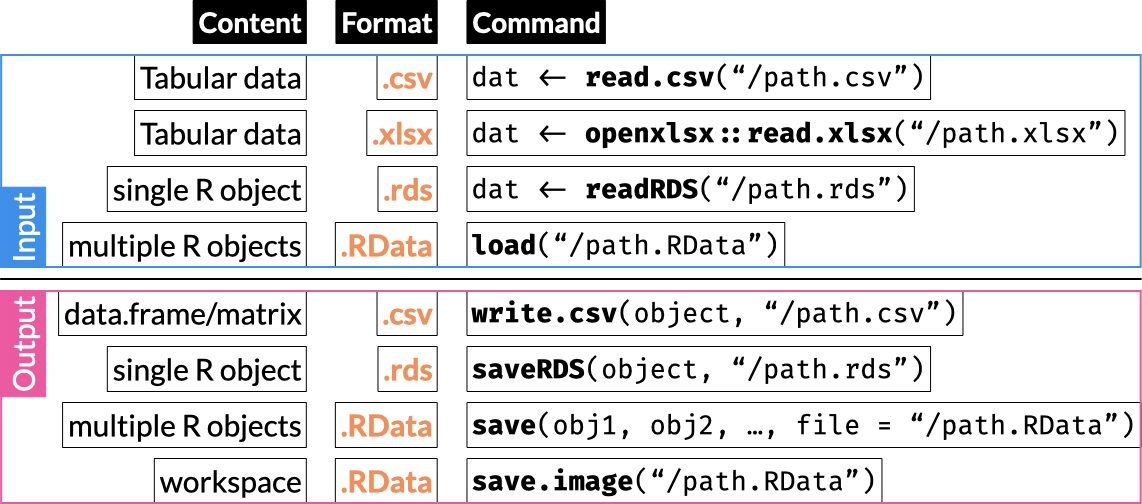
11 Base Data I/O
Tabular data typically consists of rows and columns, where the rows correspond to different cases (e.g. patients) and the columns correspond to different variables a.k.a. covariates a.k.a. features. Such data can be stored in multiple different file formats.
This includes plain text files, often in a delimited format, and binary files.
Common delimited format files includes comma- and tab-separated values (CSV, TSV).
Binary file formats can be either open (e.g. R’s RDS format) or proprietary (e.g. Microsoft’s XLS).
R includes built-in support for reading and writing multiple file formats, including delimited format files and its own binary RDS and RData files.
Third party packages add support for working with virtually any file type.
11.1 CSV
11.1.1 Read local CSV
read.table() is the core function that reads data from formatted text files in R, where cases correspond to lines and variables to columns. Its many arguments allow to read different formats. read.csv() is an alias for read.table() that defaults to commas as separators and dots for decimal points. (Run read.csv in the console to print its source read the documentation with ?read.table).
Some important arguments for read.table() listed here with their default values for read.csv():
-
sep = ",": Character that separate entries. Default is a comma; usesep = "\t"for tab-separated files (default setting inread.delim()) -
dec = ".": Character for the decimal point. Default is a dot; in some cases where a comma is used as the decimal point, the entry separatorsepmay be a semicolon (default setting inread.csv2()) -
na.strings = "NA": Character vector of strings to be coded as “NA” -
colClasses = NA: Either a character vector defining each column’s type (e.g.c("character", "numeric", "numeric")recycled as necessary or a named vector defining specific columns’ types (e.g.c(ICD9 = "character", Sex = "factor", SBP = "numeric", DOB = "Date")). Unspecified columns are automatically determined. Note: Set a column to"NULL"(with quotes) to exclude that column. -
stringsAsFactors = TRUE: Will convert all character vectors to factors
men <- read.csv("../Data/pone.0204161.s001.csv")
Note
When working in Windows, paths should use either single forward slashes (/) or double backslashes (\\).
11.1.2 Read CSV from the web
read.csv() can directly read an online file. In the second example below, we also define that missing data is coded with ? using the na.strings argument:
hf <- read.csv("https://archive.ics.uci.edu/ml/machine-learning-databases/00519/heart_failure_clinical_records_dataset.csv"The above file is read directly from the UCI ML repository (See data repositories).
11.1.3 Read zipped data from the web
11.1.3.1 using gzcon() and read.csv()
read.table() /read.csv() also accepts a “connection” as input.
Here we define a connection to a zipped file by nesting gzcon() and url():
We read the connection and specify the file is tab-separated, or call read.delim():
bcw <- read.csv(con, header = TRUE, sep = "\t")

#same as
bcw <- read.delim(con, header = TRUE)
11.1.4 Write to CSV
Use the write.csv() function to write an R object (usually data frame or matrix) to a CSV file. Setting row.names = FALSE is usually a good idea. (Instead of storing data in rownames, it’s usually best to create a new column.)
write.csv(iris, "../Data/iris.csv", row.names = FALSE)Note that in this case we did not need to save row names (which are just integers 1 to 150 and would add a useless extra column in the output)
11.2 Excel .XLSX files
Two popular packages to read Excel files are openxlsx and readxl.
11.3 Read .xslx
11.3.1 openxlsx::read.xlsx()
NA strings are defined with argument na.strings.
bcw <- openxlsx::read.xlsx("../Data/bcw.xlsx", na.strings = ".")
11.3.2 readxl::read_xlsx()
NA strings are defined with argument na.
bcw <- readxl::read_xlsx("../Data/bcw.xlsx", na = ".")11.4 Write .xlsx
11.4.1 openxlsx::write.xlsx()
openxlsx::write.xlsx(bcw, "../Data/bcw.xlsx")Note: The readxl package does not include a function to write .XLSX files.
11.5 RDS
11.5.1 Read single R object from an RDS file
To load an object saved in an RDS file, you read it with readRDS() and must assign it to an object:
To read an RDS file directly from a web server, you surround the URL with url():
11.5.2 Write single R object to an RDS file
You can write any single R object as an RDS file so that you can recover it later, share it, etc. Remember that since a list can contain any number of objects of any type, you can save essentially any collection of objects in an RDS file.
For multiple objects, see also the save.image() command below.
saveRDS(bcw, "bcw.rds")11.6 RData
11.6.1 Write multiple R objects to an RData file
You can use the save() function to save multiple R objects to a single .RData file:
Note: we will learn how to use sapply() later under Loop functions
To load the variables in the RData file you saved, use the load() command:
load("./mat.RData")Note that load() adds the objects to your workspace using their original names. You do not assign them to a new object, unlike with the readRDS() call above.
11.6.2 Write your entire workspace to an RData file
You can save your entire workspace to a RData file using the save.image() function:
save.image("workspace_2022-08-10.RData")11.6.3 Load .Rdata
Same as above, to re-load the workspace saved in the .RData file, use the load() command:
load("workspace_2022-08-10.RData")11.7 System commands
Get working directory with getwd():
getwd()Set the working directory with setwd():
setwd("/Data/")You can set a different working directory with setwd().
List files in current directory:
dir()You can send operating system commands using system():
system("uname -a")Note: See issue here.
11.8 Read other common tabular data third-party formats
| File type | File Extension | package::function() |
|---|---|---|
| JSON | .json |
jsonlite::read_json() |
| Stata data | .dta |
haven::read_dta() |
| SPSS data |
.por, .sav, .zsav
|
haven::read_spss() |
| SAS transport file | .xpt |
haven::read_xpt() |
| Matlab data | .mat |
rmatio::read.mat() |
| Apache Arrow | .arrow |
arrow::read_arrow() |
| Apache Arrow | .feather |
arrow::read_feather() |
| Apache Arrow | .parquet |
arrow::read_parquet() |
| Weka ARFF | .arff |
farff::readARFF() |
11.9 See also
11.10 Resources
- R Data Import/Export by the R Core Team.