48 Optimization
R provides a general purpose optimization tool, optim(). You can use it to estimate parameters that minimize any defined function.
Supervised and unsupervised learning involves defining a loss function to minimize or an objective function to minimize or maximize.
To learn how optim() works, let’s write a simple function that returns linear coefficients by minimizing squared error.
48.1 Data
48.2 GLM (glm, s_GLM)
Call:
glm(formula = y ~ x)

Coefficients:
             Estimate Std. Error t value Pr(>|t|)
(Intercept) 11.979070   0.043252 276.962   <2e-16 ***
x1           0.061798   0.040916   1.510   0.1316
x2          -0.003873   0.043271  -0.090   0.9287
x3           1.488113   0.042476  35.034   <2e-16 ***
x4           0.031115   0.044015   0.707   0.4800
x5           0.034217   0.043664   0.784   0.4336
x6           0.034716   0.042189   0.823   0.4110
x7           3.183398   0.040605  78.399   <2e-16 ***
x8          -0.034252   0.043141  -0.794   0.4276
x9           0.541219   0.046550  11.627   <2e-16 ***
x10          0.087120   0.044000   1.980   0.0483 *
---
Signif. codes:  0 '***' 0.001 '**' 0.01 '*' 0.05 '.' 0.1 ' ' 1

(Dispersion parameter for gaussian family taken to be 0.9207315)

    Null deviance: 7339.42  on 499  degrees of freedom
Residual deviance:  450.24  on 489  degrees of freedom
AIC: 1390.5

Number of Fisher Scoring iterations: 2
Or, using rtemis:
mod.glm <- s_GLM(x, y)09-28-23 21:49:28 Hello, egenn [s_GLM]
.:Regression Input Summary
Training features: 500 x 10
Training outcome: 500 x 1
Testing features: Not available
Testing outcome: Not available
09-28-23 21:49:29 Training GLM... [s_GLM]
.:GLM Regression Training Summary
MSE = 0.90 (93.87%)
RMSE = 0.95 (75.23%)
MAE = 0.77 (74.88%)
r = 0.97 (p = 5.3e-304)
R sq = 0.94
09-28-23 21:49:29 Completed in 0.01 minutes (Real: 0.42; User: 0.38; System: 0.02) [s_GLM]
summary(mod.glm$mod)
Call:
glm(formula = .formula, family = family, data = df.train, weights = .weights,
    na.action = na.action)

Coefficients:
             Estimate Std. Error t value Pr(>|t|)
(Intercept) 11.979070   0.043252 276.962   <2e-16 ***
V1           0.061798   0.040916   1.510   0.1316
V2          -0.003873   0.043271  -0.090   0.9287
V3           1.488113   0.042476  35.034   <2e-16 ***
V4           0.031115   0.044015   0.707   0.4800
V5           0.034217   0.043664   0.784   0.4336
V6           0.034716   0.042189   0.823   0.4110
V7           3.183398   0.040605  78.399   <2e-16 ***
V8          -0.034252   0.043141  -0.794   0.4276
V9           0.541219   0.046550  11.627   <2e-16 ***
V10          0.087120   0.044000   1.980   0.0483 *
---
Signif. codes:  0 '***' 0.001 '**' 0.01 '*' 0.05 '.' 0.1 ' ' 1

(Dispersion parameter for gaussian family taken to be 0.9207315)

    Null deviance: 7339.42  on 499  degrees of freedom
Residual deviance:  450.24  on 489  degrees of freedom
AIC: 1390.5

Number of Fisher Scoring iterations: 2
48.3 optim()
Basic usage of optim to find values of parameters that minimize a function:
- Define a list of initial parameter values
- Define a loss function whose first argument is the above list of initial parameter values
- Pass parameter list and objective function to
optim
In the following example, we wrap these three steps in a function called linearcoeffs, which will output the linear coefficients that minimize squared error, given a matrix/data.frame of features x and an outcome y. We also specify the optimization method to be used (See ?base::optim for details):
linearcoeffs <- function(x, y, method = "BFGS") {

  # 1. List of initial parameter values
  params <- as.list(c(mean(y), rep(0, NCOL(x))))
  names(params) <- c("Intercept", paste0("Coefficient", seq(NCOL(x))))

  # 2. Loss function: first argument is parameter list
  loss <- function(params, x, y) {
    estimated <- c(params[[1]] + x %*% unlist(params[-1]))
    mean((y - estimated)^2)
  }

  # 3. optim!
  coeffs <- optim(params, loss, x = x, y = y, method = method)

  # The values that minimize the loss function are stored in $par
  coeffs$par
}
coeffs.optim <- linearcoeffs(x, y)
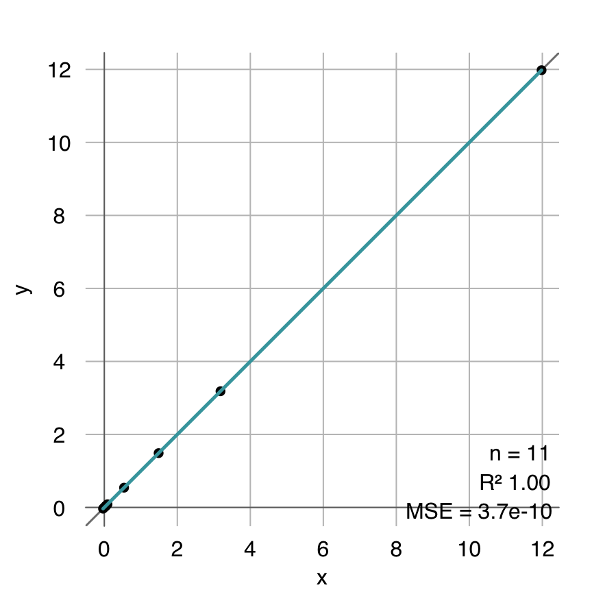
estimated.optim <- cbind(1, x) %*% coeffs.optim
mplot3_fit(y, estimated.optim)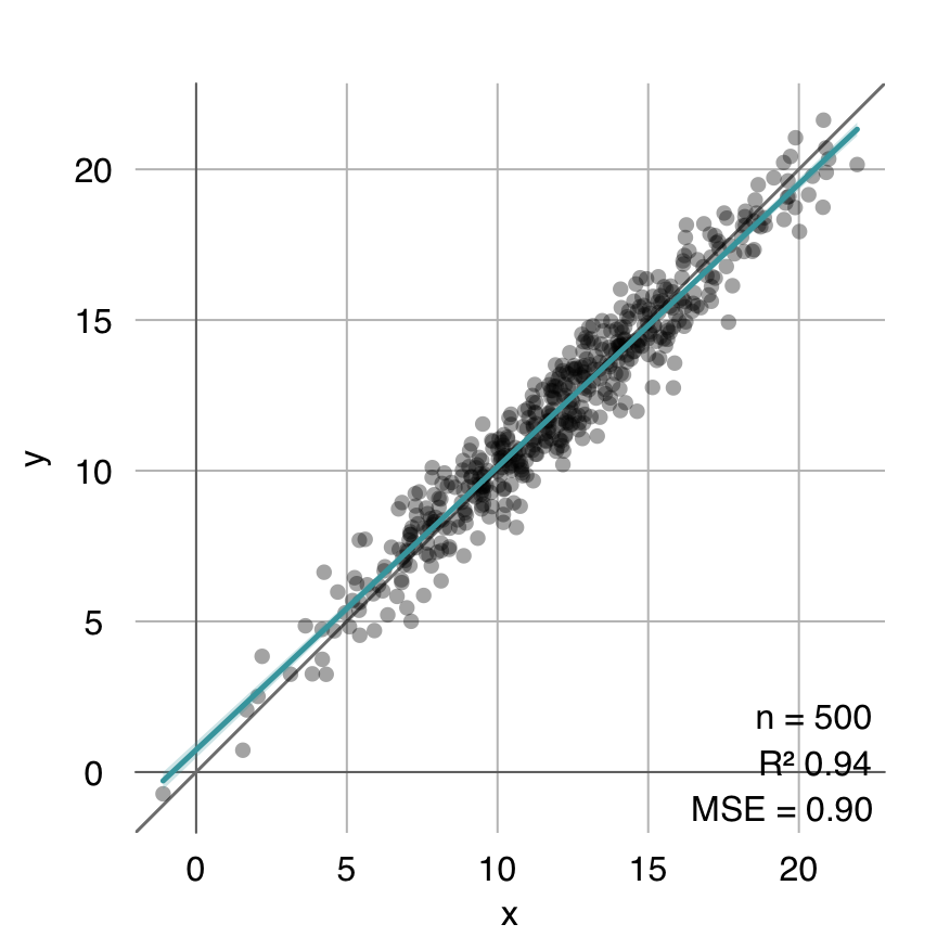
coeffs.glm <- mod.glm$mod$coefficients
estimated.glm <- cbind(1, x) %*% coeffs.glm
mplot3_fit(y, estimated.glm)
mplot3_fit(coeffs.glm, coeffs.optim)